2.5D Training - Unleashing 3D Power on a 2D Budget

Introduction

In this project I’ll design a model that automatically segments the stomach and intestines in MRI scans for cancer patient care. The MRI scans originate from cancer patients who underwent 1-5 MRI scans on separate days during their radiation treatment. The algorithm I’m developing relies on a dataset of these scans, aiming to innovate deep learning solutions that will improve patient outcomes. A significant aspect of this project involves a technique known as 2.5D imaging, which merges the power of 3D imaging with the simplicity and efficiency of 2D resources.

MRI scans of 2D and 2.5 images

Dataset Description

The competition utilizes RLE-encoded masks for training annotations, with images presented in 16-bit grayscale PNG format. Each case is represented by multiple sets of scan slices, with some cases split by time, others by case, urging the development of a model that generalizes to both partially and wholly unseen cases.

The Magic of 2.5D Imaging

2.5D image creation.

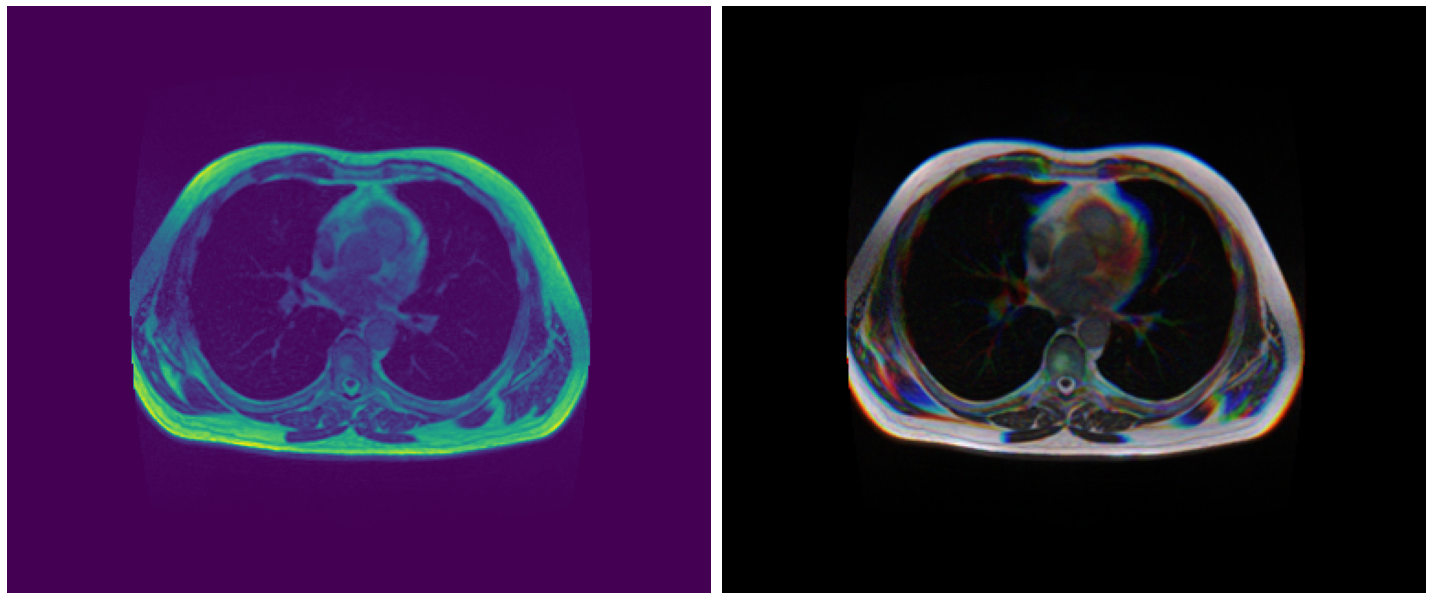
While 2D training on MRI scans is relatively straightforward, the depth information in the MRI slices opens up a whole new world of possibilities. By stacking consecutive slices, we can form what appears to be a 3D volume. However, I dub this process 2.5D imaging, because we train these 3D-like images as if they were 2D.

In a regular 2D training scenario, such as with RGB images, we pass a 3D tensor (e.g., [None, channel, height, width]) to a model. In PyTorch, the last two dimensions represent the spatial aspects (height & width), and the first one is the channel dimension. But in the case of MRI images, where channel information is absent, we can use that dimension to stack multiple MRI scans as channels and train them as 2D images.

This 2.5D method brings with it a raft of benefits over traditional 3D training:

Lower GPU/memory cost
Simplified pipeline
Easier augmentation
More straightforward inference
Wide availability of open-source models

The result mirrors a 3D movie scene in the theater, as illustrated above. The advantages of this approach manifest in the impressive lb & cv scores achieved, probably owing to the extra depth information obtained through stacking multiple consecutive slices in channels.

In my approach, to maintain aspect ratios and prevent data loss, I have opted for padding instead of resizing images. Hence, the training image size stands at 320x384. You can explore this further in my notebook.

How to Implement 2.5D Imaging

Utility Functions

# Load Image
def load_img(path, size=IMG_SIZE):
    img = cv2.imread(path, cv2.IMREAD_UNCHANGED)
    shape0 = np.array(img.shape[:2])
    resize = np.array(size)
    if np.any(shape0!=resize):
        diff = resize - shape0
        pad0 = diff[0]
        pad1 = diff[1]
        pady = [pad0//2, pad0//2 + pad0%2]
        padx = [pad1//2, pad1//2 + pad1%2]
        img = np.pad(img, [pady, padx])
        img = img.reshape((*resize))
    return img

# Load Mask with .npy format
def load_msk(path, size=IMG_SIZE):
    msk = np.load(path)
    shape0 = np.array(msk.shape[:2])
    resize = np.array(size)
    if np.any(shape0!=resize):
        diff = resize - shape0
        pad0 = diff[0]
        pad1 = diff[1]
        pady = [pad0//2, pad0//2 + pad0%2]
        padx = [pad1//2, pad1//2 + pad1%2]
        msk = np.pad(msk, [pady, padx, [0,0]])
        msk = msk.reshape((*resize, 3))
    return msk

# Load multiple images
def load_imgs(img_paths, size=IMG_SIZE):
    imgs = np.zeros((*size, len(img_paths)), dtype=np.uint16)
    for i, img_path in enumerate(img_paths):
        img = load_img(img_path, size=size)
        imgs[..., i]+=img
    return imgs

Extract Meta Data

df = pd.read_csv('../input/uwmgi-mask-dataset/train.csv')
df['segmentation'] = df.segmentation.fillna('')
df['rle_len'] = df.segmentation.map(len) # length of each rle mask
df['mask_path'] = df.mask_path.str.replace('/png/','/np').str.replace('.png','.npy')

df2 = df.groupby(['id'])['segmentation'].agg(list).to_frame().reset_index() # rle list of each id
df2 = df2.merge(df.groupby(['id'])['rle_len'].agg(sum).to_frame().reset_index()) # total length of all rles of each id

df = df.drop(columns=['segmentation', 'class', 'rle_len'])
df = df.groupby(['id']).head(1).reset_index(drop=True)
df = df.merge(df2, on=['id'])
df['empty'] = (df.rle_len==0) # empty masks
df.head()

Create 2.5D Images (This is where the magic happens!)

channels=3
stride=2
for i in range(channels):
    df[f'image_path_{i:02}'] = df.groupby(['case','day'])['image_path'].shift(-i*stride).fillna(method="ffill")
df['image_paths'] = df[[f'image_path_{i:02d}' for i in range(channels)]].values.tolist()
df.image_paths[0]

Display 2.5D Images

idx = 40

plt.figure(figsize=(20, 10))
plt.subplot(1, 2, 1)
img = load_img(df.image_path[idx]).astype('float32')
img/=img.max()
plt.imshow(img); plt.axis('off')


plt.subplot(1, 2, 2)
imgs = load_imgs(df.image_paths[idx]).astype('float32')
imgs/=imgs.max(axis=(0,1))
plt.imshow(imgs); plt.axis('off')

plt.tight_layout()
plt.show()